Illustrating multivariate MAPIT with Simulated Data
Julian Stamp
2026-02-20
Source:vignettes/mvMAPIT.Rmd
mvMAPIT.RmdNote: For univariate analyses (single trait), check out the much faster implementation: Sparse Modeling of Epistasis (SME)
Please Cite Us
If you use multivariate MAPIT in published research, please cite:
Crawford L, Zeng P, Mukherjee S, & Zhou X (2017). Detecting epistasis with the marginal epistasis test in genetic mapping studies of quantitative traits. PLoS genetics, 13(7), e1006869. https://journals.plos.org/plosgenetics/article?id=10.1371/journal.pgen.1006869
Stamp J, DenAdel A, Weinreich D, Crawford, L (2023). Leveraging the Genetic Correlation between Traits Improves the Detection of Epistasis in Genome-wide Association Studies. G3 Genes|Genomes|Genetics 13(8), jkad118; doi: https://doi.org/10.1093/g3journal/jkad118
Stamp J, Pattillo Smith S, Weinreich D, Crawford L (2025). Sparse modeling of interactions enables fast detection of genome-wide epistasis in biobank-scale studies. The American Journal of Human Genetics, 112(9), 2198-2212; doi: https://doi.org/10.1016/j.ajhg.2025.07.004
Stamp J, Crawford L (2022). mvMAPIT: Multivariate Genome Wide Marginal Epistasis Test. https://github.com/lcrawlab/mvMAPIT, https://lcrawlab.github.io/mvMAPIT/
Getting Started
Load necessary libraries. For the sake of getting started,
mvMAPIT comes with a small set of simulated data. This data
contains random genotype-like data and two simulated quantitative traits
with epistatic interactions. To make use of this data, call the genotype
data as simulated_data$genotype, and the simulated trait
data as simulated_data$trait. The vignette traces the
analysis of simulated data. The simulations are described in
vignette("simulations").
For a working installation of mvMAPIT please look at
theREADME.md or vignette("docker-mvmapit")
Running mvMAPIT
The R routine mvmapit can be run in multiple modes. By
default it runs in a hybrid mode, performing tests both wtih a normal
Z-test as well as the Davies method. The resulting p-values
can be combined using functions provided by mvMAPIT,
e.g. fishers_combined(), that work on the
pvalues tibble that mvmapit returns.
NOTE: mvMAPIT takes the X matrix as ; not as .
mvmapit_hybrid <- mvmapit(
        t(data$genotype),
        t(data$trait),
        test = "hybrid"
)
fisher <- fishers_combined(mvmapit_hybrid$pvalues)
To visualize the genome wide p-values, we use a
Manhattan plot. The p-values are plotted after combining
the results from the multivariate analysis using Fisher’s method.
manhplot <- ggplot(fisher, aes(x = 1:nrow(fisher), y = -log10(p))) +
  geom_hline(yintercept = -log10(thresh), color = "grey40", linetype = "dashed") +
  geom_point(alpha = 0.75, color = "grey50") +
  geom_text_repel(aes(label=ifelse(p < thresh, as.character(id), '')))
plot(manhplot)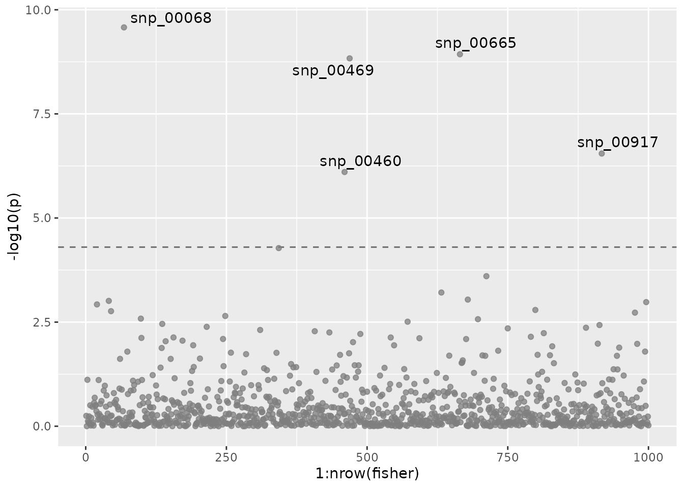
To control the type I error despite multiple testing, we recommend
the conservative Bonferroni correction. The significant SNPs returned by
the mvMAPIT analysis are shown in the output below. There
are in total 6 significant SNPs after multiple test correction. Of the
significant SNPs, 4 are true positives.
thresh <- 0.05 / nrow(fisher)
significant_snps <-  fisher %>%
    filter(p < thresh) # Call only marginally significant SNPs

truth <- simulated_data$epistatic %>%
  ungroup() %>%
  mutate(discovered = (name %in% significant_snps$id)) %>%
  select(name, discovered) %>%
  unique()

significant_snps %>%
  mutate_if(is.numeric, ~(as.character(signif(., 3)))) %>%
  mutate(true_pos = id %in% truth$name) %>%
  kable(., linesep = "") %>%
kable_material(c("striped"))| id | trait | p | true_pos |
|---|---|---|---|
| snp_00068 | fisher | 2.65e-10 | TRUE |
| snp_00460 | fisher | 7.86e-07 | FALSE |
| snp_00469 | fisher | 1.47e-09 | TRUE |
| snp_00665 | fisher | 1.17e-09 | TRUE |
| snp_00917 | fisher | 2.83e-07 | TRUE |
True Epistatic SNPs
To compare this list to the full list of causal epistatic SNPs of the simulations, refer to the following list. There are 5 causal SNPs. Of these 5 causal SNPs, 4 were succesfully discovered by mvMAPIT.
truth %>%
  kable(., linesep = "") %>%
kable_material(c("striped"))| name | discovered |
|---|---|
| snp_00068 | TRUE |
| snp_00156 | FALSE |
| snp_00469 | TRUE |
| snp_00665 | TRUE |
| snp_00917 | TRUE |
Running an Informed Exhaustive Search
Now we may take only the significant SNPs according to their marginal epistatic effects and run a simple exhaustive search between them.
The search itself is a simple regression on the interaction terms between all significant interactions.
# exhaustive search for p-values
pairs <- NULL
if (nrow(significant_snps) > 1) {
  pairnames <- comboGeneral(significant_snps$id, 2)
  # Generate unique pairs of SNP names;
  # for length(names) = n, the result is a (n * (n-1)) x 2 matrix with one row corresponding to a pair
  for (k in seq_len(nrow(pairnames))) {
    fit <- lm(y ~ X[, pairnames[k, 1]]:X[, pairnames[k, 2]])
    p_value1 <- coefficients(summary(fit))[[1]][2, 4]
    p_value2 <- coefficients(summary(fit))[[2]][2, 4]
    tib <- dplyr::tibble(
            x = p_value1,
            y = p_value2,
            u = pairnames[k, 1],
            v = pairnames[k, 2]
    )
    pairs <- bind_rows(pairs, tib)
  }
}

colnames(pairs) <- c(colnames(y), "var1", "var2")
Visualize Exhaustive Search Results
We plot the
of the p-values for the regression coefficients as tile
plot to highlight the identified interaction structure.
plotable <- pairs %>%
  pivot_longer(
    cols = starts_with("p_"),
    names_to = "trait",
    names_prefix = "trait ",
    values_to = "p",
    values_drop_na = TRUE
  ) %>%
  mutate(trait = case_when(
    trait == "p_01" ~ "Trait 1",
    trait == "p_02"  ~ "Trait 2"))
tiles <- ggplot(data = plotable, aes(x=var1, y=var2, fill=-log10(p)))+
  geom_tile() +
  facet_wrap(~trait) +
  theme(axis.text.x = element_text(angle = 90, vjust = 0.5, hjust=1)) +
  scale_fill_viridis_c()
plot(tiles)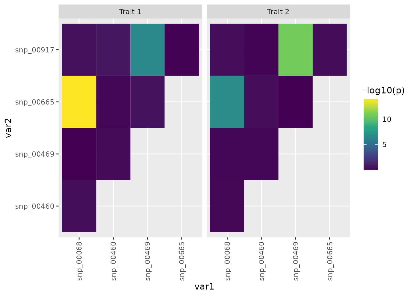
The only significant interactions after multiple testing correction
are the interaction between snp00068 and
snp_00665 as well as snp_00469 and
snp_00917.
pairs %>%
  filter(p_01 < 0.05/nrow(pairs) | p_02 < 0.05/nrow(pairs)) %>%
  kable(., linesep = "", digits = 14) %>%
kable_material(c("striped"))| p_01 | p_02 | var1 | var2 |
|---|---|---|---|
| 1.000000e-14 | 1.645102e-07 | snp_00068 | snp_00665 |
| 2.640252e-07 | 1.559000e-11 | snp_00469 | snp_00917 |
True epistataic structure
Compare the results of the exhaustive search to the true interaction structure. Notice that the only significant interactions in the exhaustive search are the two with the largest true effects.
true_interactions <- simulated_data$interactions %>%
  mutate(var1 = sprintf(group1, fmt = "snp_%05d")) %>%
  mutate(var2 = sprintf(group2, fmt = "snp_%05d")) %>%
  mutate(trait = case_when(
    trait == 1 ~ "Trait 1",
    trait == 2  ~ "Trait 2")) %>%
  select(-c("group1", "group2"))
X <- true_interactions[, c("var1", "var2")]
X  <- t(apply(X, 1, sort))
true_interactions[,c("var1", "var2")]  <- X

epistatic_pairnames <- comboGeneral(simulated_data$epistatic$name %>% unique(), 2)
true_pairs <- NULL
for (k in seq_len(nrow(epistatic_pairnames))) {
  tib <- dplyr::tibble(var1 = epistatic_pairnames[k, 1],
                        var2 = epistatic_pairnames[k, 2])
  true_pairs <- bind_rows(true_pairs, tib)
}
anti <- anti_join(true_pairs, true_interactions) %>%
  mutate(effect_size = 0)
# Joining with `by = join_by(var1, var2)`

true_int_plot <- true_interactions %>%
  bind_rows(anti %>% mutate(trait = "Trait 1")) %>%
  bind_rows(anti %>% mutate(trait = "Trait 2"))

true_tiles <- ggplot(data = true_int_plot, aes(x=var1, y=var2, fill=effect_size)) +
  geom_tile() +
  facet_wrap(~trait) +
  theme(axis.text.x = element_text(angle = 90, vjust = 0.5, hjust=1)) +
  scale_fill_gradient2(low = "blue", high = "red", mid = "white")
plot(true_tiles)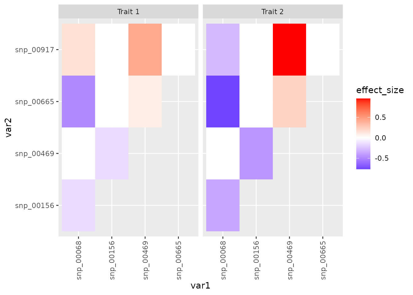
While mvMAPIT does not identify the explicit partner, it still implicates more correct SNPs in this example. All true epistatic SNPs are listed in the following table.
true_interactions %>%
  kable(., linesep = "") %>%
kable_material(c("striped"))| effect_size | trait | var1 | var2 |
|---|---|---|---|
| -0.1446703 | Trait 1 | snp_00156 | snp_00469 |
| -0.1463573 | Trait 1 | snp_00068 | snp_00156 |
| 0.0876213 | Trait 1 | snp_00469 | snp_00665 |
| -0.4940839 | Trait 1 | snp_00068 | snp_00665 |
| 0.4244533 | Trait 1 | snp_00469 | snp_00917 |
| 0.1504647 | Trait 1 | snp_00068 | snp_00917 |
| -0.4336821 | Trait 2 | snp_00156 | snp_00469 |
| -0.3663968 | Trait 2 | snp_00068 | snp_00156 |
| 0.2189245 | Trait 2 | snp_00469 | snp_00665 |
| -0.7666908 | Trait 2 | snp_00068 | snp_00665 |
| 0.9583180 | Trait 2 | snp_00469 | snp_00917 |
| -0.2884704 | Trait 2 | snp_00068 | snp_00917 |