15. Marker Gene Method Comparison (Supplemental Figure S39)
15_S39_DE_comparison.Rmd
suppressPackageStartupMessages({
library(ggplot2)
library(ggVennDiagram)

library(Seurat)})
library(countsplit)
library(ClusterDE)
We begin by defining several functions. First, the clusterDE workflow.
clusterDE_workflow <- function(seurat_obj, cluster1, cluster2, cores) {
  set.seed(1)

  original_markers <- FindMarkers(seurat_obj,
                                  ident.1 = cluster1,
                                  ident.2 = cluster2,
                                  min.pct = 0,
                                  logfc.threshold = 0)

  seurat_obj_sub <- subset(x = seurat_obj, idents = c(cluster1, cluster2))
  count_mat <- GetAssayData(object = seurat_obj_sub, slot = "counts")
  synthetic_null <- ClusterDE::constructNull(count_mat, nCores = cores, fastVersion = TRUE)

  seurat_obj_null <- CreateSeuratObject(counts = synthetic_null)
  seurat_obj_null <- NormalizeData(seurat_obj_null)
  seurat_obj_null <- FindVariableFeatures(object = seurat_obj_null)
  seurat_obj_null <- ScaleData(object = seurat_obj_null)
  seurat_obj_null <- RunPCA(object = seurat_obj_null)
  seurat_obj_null <- FindNeighbors(object = seurat_obj_null)

  resolution <- 0.1
  while (length(levels(Idents(seurat_obj_null))) == 1) {
    resolution <- resolution + 0.1
    seurat_obj_null <- FindClusters(object = seurat_obj_null, resolution = resolution)
    print("Num clusters")
    print(length(levels(Idents(seurat_obj_null))))
  }

  null_markers <- FindMarkers(seurat_obj_null,
                              ident.1 = 0,
                              ident.2 = 1,
                              min.pct = 0,
                              logfc.threshold = 0)

  original_pval <- original_markers$p_val
  names(original_pval) <- rownames(original_markers)

  null_pval <- null_markers$p_val
  names(null_pval) <- rownames(null_markers)

  res <- ClusterDE::callDE(original_pval, null_pval, nlogTrans = TRUE, FDR = 0.05)

  return(res)
}
Then we write a function for the countsplit workflow.
countsplit_workflow <- function(seurat_obj) {
  set.seed(1)

  counts_mat <- GetAssayData(seurat_obj, "RNA")

  split <- countsplit(counts_mat)
  Xtrain <- split[[1]]
  Xtest <- split[[2]]

  seurat_obj_train <- Seurat::CreateSeuratObject(counts = Xtrain)
  seurat_obj_test <- Seurat::CreateSeuratObject(counts = Xtest)


  # process training data
  seurat_obj_train <- Seurat::NormalizeData(seurat_obj_train,
                                            verbose = FALSE)

  seurat_obj_train <- Seurat::FindVariableFeatures(seurat_obj_train,
                                                   selection.method = "vst",
                                                   verbose = FALSE)

  seurat_obj_train <- Seurat::ScaleData(seurat_obj_train, verbose = FALSE)
  seurat_obj_train <- Seurat::RunPCA(seurat_obj_train,
                                     features = Seurat::VariableFeatures(object = seurat_obj_train),
                                     verbose = FALSE)

  seurat_obj_train <- Seurat::FindNeighbors(seurat_obj_train,
                                            verbose = FALSE)


  seurat_obj_train <- Seurat::FindClusters(seurat_obj_train,
                                            resolution = 0.8,
                                            verbose = FALSE)

  seurat_obj_train <- Seurat::RunUMAP(seurat_obj_train, dims=1:10)


  seurat_obj_test <- Seurat::NormalizeData(seurat_obj_test,
                                           verbose = FALSE)

  seurat_obj_test <- Seurat::FindVariableFeatures(seurat_obj_test,
                                                  selection.method = "vst",
                                                  verbose = FALSE)

  seurat_obj_test <- Seurat::ScaleData(seurat_obj_test, verbose = FALSE)

  seurat_obj_test <- Seurat::RunPCA(seurat_obj_test,
                                     features = Seurat::VariableFeatures(object = seurat_obj_test),
                                     verbose = FALSE)

  seurat_obj_test <- Seurat::FindNeighbors(seurat_obj_test,
                                            verbose = FALSE)

  seurat_obj_test <- Seurat::RunUMAP(seurat_obj_test, dims=1:10)

  Idents(seurat_obj_test) <- Idents(seurat_obj_train)
  seurat_obj_test@meta.data$cell_ontology_class <- seurat_obj@meta.data$cell_ontology_class

  seurat_obj_train@meta.data$cell_ontology_class <- seurat_obj@meta.data$cell_ontology_class


  return(list("seurat_obj_train"=seurat_obj_train, "seurat_obj_test"=seurat_obj_test))
}
We write function for plotting the UMAPs.
DE_comparisons_scatter_plots <- function(tissue, tissue_name, legend_pos=c(0.2, 0.2)) {
  louvain_default <- custom_scatter(tissue, "umap", group_by = "seurat_clusters", x_title = "UMAP 1", y_title = "UMAP 2", pt.size = 2, label=FALSE) #+ Seurat::NoLegend()
  louvain_recall <- custom_scatter(tissue, "umap", group_by = "recall_idents", x_title = "UMAP 1", y_title = "UMAP 2", pt.size = 2) #+ Seurat::NoLegend()
  louvain_countsplit <- custom_scatter(tissue, "umap", group_by = "countsplit_idents", x_title = "UMAP 1", y_title = "UMAP 2", pt.size = 2) #+ Seurat::NoLegend()
  cell_ontology <- custom_scatter(tissue, "umap", group_by = "cell_ontology_class", x_title = "UMAP 1", y_title = "UMAP 2", pt.size = 2) +
    ggplot2::theme(legend.position = legend_pos,
                   legend.text = ggplot2::element_text(size=20)) +
    ggplot2::guides(colour = ggplot2::guide_legend(override.aes = list(size=6), ncol = 1)) +
    ggplot2::scale_colour_discrete(na.translate = F)

  column_label_1 <- patchwork::wrap_elements(panel = grid::textGrob('Cell Ontology', gp = grid::gpar(fontsize = 64)))
  column_label_2 <- patchwork::wrap_elements(panel = grid::textGrob('Seurat Default', gp = grid::gpar(fontsize = 64)))
  column_label_3 <- patchwork::wrap_elements(panel = grid::textGrob('recall+ZIP', gp = grid::gpar(fontsize = 64, fontfamily = "Courier")))
  column_label_4 <- patchwork::wrap_elements(panel = grid::textGrob('countsplit', gp = grid::gpar(fontsize = 64, fontfamily = "Courier")))


  umap_grid <- column_label_1 + column_label_2 + column_label_3 + column_label_4 +
    cell_ontology + louvain_default + louvain_recall + louvain_countsplit +
    patchwork::plot_layout(widths = c(5, 5, 5, 5),
                           heights = c(1,3))

  return(umap_grid)
}
We write function for plotting the P-values.
compare_markers_p_vals <- function(default_markers_a, default_markers_b, xlabel, ylabel, title, xmax, ymax) {
  # sort genes alphabetically
  default_markers_a <- default_markers_a[ order(row.names(default_markers_a)), ]
  default_markers_b <- default_markers_b[ order(row.names(default_markers_b)), ]

  log_p_val_a <- -log(default_markers_a$p_val)
  log_p_val_b <- -log(default_markers_b$p_val)

  df <- data.frame(log_p_val_a, log_p_val_b)

  r_p_val <- cor(log_p_val_a, log_p_val_b)

  large_text_size <- 32
  small_text_size <- 24

  correlation_text_size <- 16

  p_value_scatterplot <- ggplot2::ggplot(df, ggplot2::aes(x = log_p_val_a, y = log_p_val_b)) +
    ggplot2::geom_point() +
    ggplot2::theme_bw() +
    xlim(0, xmax) +
    ylim(0, ymax) +
    ggplot2::xlab(xlabel) +
    ggplot2::ylab(ylabel) +
    ggplot2::annotate("text", x = 25, y = ymax * 0.82, label = paste0("r = ", round(r_p_val, 3)), size = correlation_text_size) +
    ggplot2::theme(axis.text = ggplot2::element_text(size = small_text_size),
                   axis.title = ggplot2::element_text(size = large_text_size),
                   plot.title = ggplot2::element_text(size = large_text_size, hjust = 0.5)) +
    ggtitle(title)

  return(p_value_scatterplot)
}
We write function for plotting the q-values.
compare_markers_q_vals <- function(default_markers_a, default_markers_b, xlabel, ylabel, title, xmax, ymax) {
  # convert clusterDE results tibble to dataframe
  default_markers_b <-  data.frame(default_markers_b)
  # make rownames the Genes
  rownames(default_markers_b) <- default_markers_b$Gene

  # sort genes alphabetically
  default_markers_a <- default_markers_a[ order(row.names(default_markers_a)), ]
  default_markers_b <- default_markers_b[ order(row.names(default_markers_b)), ]

  log_p_val_a <- -log(default_markers_a$q)
  log_p_val_b <- -log(default_markers_b$p_val)

  df <- data.frame(log_p_val_a, log_p_val_b)

  r_p_val <- cor(log_p_val_a, log_p_val_b)

  large_text_size <- 32
  small_text_size <- 24

  correlation_text_size <- 16

  p_value_scatterplot <- ggplot2::ggplot(df, ggplot2::aes(x = log_p_val_a, y = log_p_val_b)) +
    ggplot2::geom_point() +
    ggplot2::theme_bw() +
    xlim(0, xmax) +
    ylim(0, ymax) +
    ggplot2::xlab(xlabel) +
    ggplot2::ylab(ylabel) +
    ggplot2::annotate("text", x = 2, y = 340, label = paste0("r = ", round(r_p_val, 3)), size = correlation_text_size) +
    ggplot2::theme(axis.text = ggplot2::element_text(size = small_text_size),
                   axis.title = ggplot2::element_text(size = large_text_size),
                   plot.title = ggplot2::element_text(size = large_text_size, hjust = 0.5)) +
    ggtitle(title)

  return(p_value_scatterplot)
}
We write function for plotting the marker gene Venn diagram.
marker_gene_venn_diagram <- function(recall_marker_genes, countsplit_marker_genes, clusterDE_marker_genes) {
  p <- ggVennDiagram(list("recall+ZIP"=recall_marker_genes,
                          "countsplit"=countsplit_marker_genes,
                          "clusterDE"=clusterDE_marker_genes),
                     label = "count") +
    scale_fill_gradient(low = "white", high = "grey") +
    guides(fill="none") +
    scale_x_continuous(expand = expansion(mult = .2))

  return(p)
}
Now, we load the limb muscle tissue.
limb_muscle <- readRDS("Limb_Musclecluster_results_seurat.rds")
limb_muscle <- Seurat::ScaleData(limb_muscle, features = rownames(limb_muscle))

# make cell type labels a factor
limb_muscle@meta.data$cell_ontology_class <- as.factor(limb_muscle@meta.data$cell_ontology_class)
#sort cluster labels by cluster size
sorted_limb_muscle_clusters <- names(sort(summary(as.factor(na.omit(limb_muscle@meta.data$cell_ontology_class))), decreasing = TRUE))
limb_muscle@meta.data$cell_ontology_class <- factor(limb_muscle@meta.data$cell_ontology_class, levels = sorted_limb_muscle_clusters)
Now, we run the countsplit workflow.
countsplit_res <- countsplit_workflow(limb_muscle)


limb_muscle_test <- countsplit_res$seurat_obj_test

limb_muscle@meta.data$countsplit_idents <- Idents(limb_muscle_test)
Plot the UMAP of different clusterings used in this figure.
umap_grid <- DE_comparisons_scatter_plots(limb_muscle, "Limb Muscle")

ggsave("DE_marker_comparison_umap_grid.png", umap_grid, width = 36, height = 10, units = "in")
Get marker genes for recall and countsplit
# for countsplit cluster 0 is "skeletal muscle satellite cell" and cluster 1 is "mesenchymal stem cell"
countsplit_markers_0vs1 <- FindMarkers(limb_muscle_test, ident.1 = 0, ident.2 = 1, min.pct = 0, logfc.threshold = 0)

# for recall cluster 0 is "skeletal muscle satellite cell" and cluster 1 is "mesenchymal stem cell"
recall_markers_0vs1 <- FindMarkers(limb_muscle, ident.1 = 0, ident.2 = 1, group.by = "recall_idents", min.pct = 0, logfc.threshold = 0)
Run the ClusterDE workflow
# for seurat default cluster 1 is "skeletal muscle satellite cell" and cluster 2 is "mesenchymal stem cell"
clusterDE_res <- clusterDE_workflow(limb_muscle, 1, 2, cores=1)
Plot the p-value and q-value scatterplots.
countsplit_vs_recall_markers_plot <- compare_markers_p_vals(countsplit_markers_0vs1,
                                                              recall_markers_0vs1,
                                                              xlabel = "countsplit -log P-values",
                                                              ylabel = "recall+ZIP -log P-values",
                                                              title = "Skeletal muscle satellite cell cluster vs\nMesenchymal stem cell cluster",
                                                              xmax = 200,
                                                              ymax = 400)


clusterDE_vs_recall_markers_plot <- compare_markers_q_vals(clusterDE_res$summaryTable, recall_markers_0vs1,
                                                             "clusterDE -log q-values",
                                                             "recall+ZIP -log P-values",
                                                             "Skeletal muscle satellite cell cluster vs\nMesenchymal stem cell cluster",
                                                             xmax = 10,
                                                             ymax = 400)


ggsave("countsplit_vs_recall_markers_plot.png", countsplit_vs_recall_markers_plot, width = 12, height = 12, units = "in")
ggsave("clusterDE_vs_recall_markers_plot.png", clusterDE_vs_recall_markers_plot, width = 12, height = 12, units = "in")
Plot the Venn diagram
countsplit_signficant <- countsplit_markers_0vs1[countsplit_markers_0vs1$p_val_adj < 0.05, ]
recall_signficant <- recall_markers_0vs1[recall_markers_0vs1$p_val_adj < 0.05, ]

marker_venn_diagram <- marker_gene_venn_diagram(rownames(recall_signficant), rownames(countsplit_signficant), clusterDE_res$DEgenes)

ggsave("marker_venn_diagram.png", marker_venn_diagram)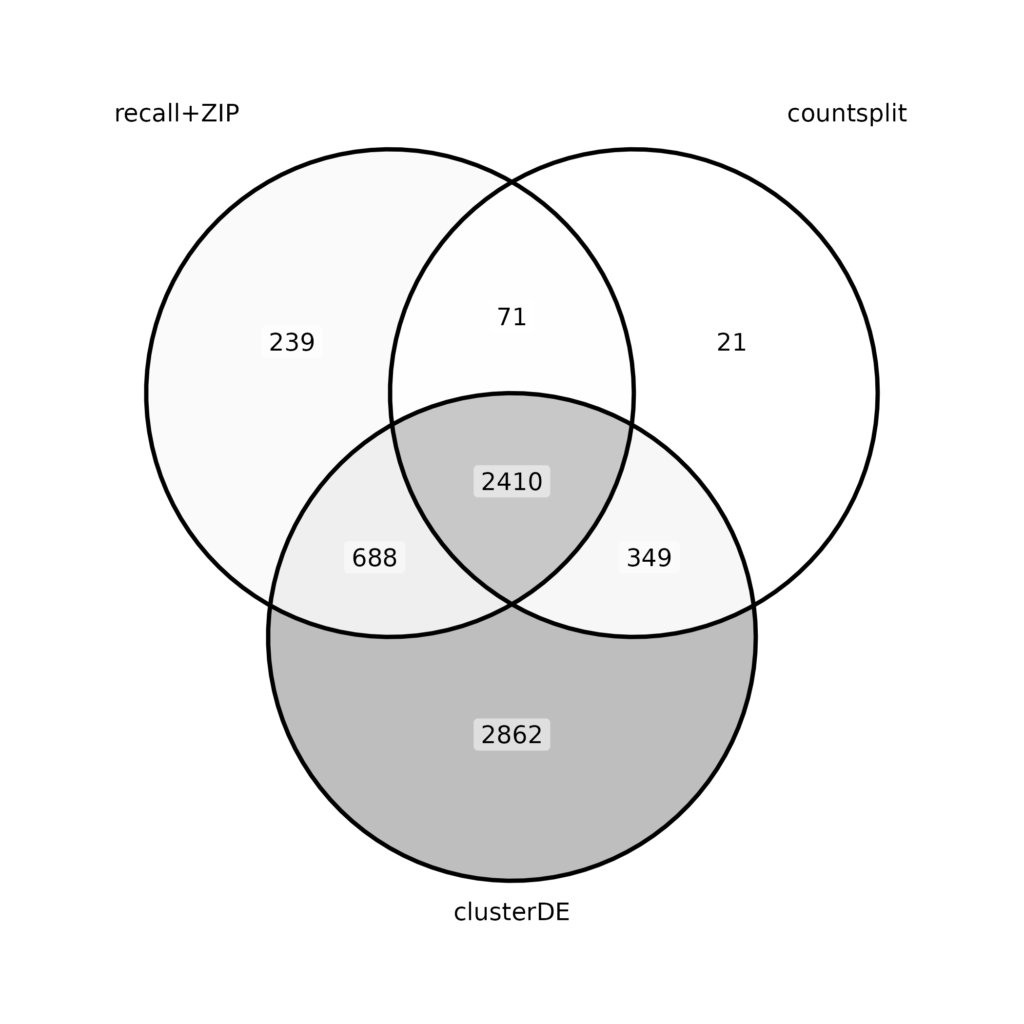
Finally, we plot the P-value comparison for recall and countsplit with recall clusters downsampled.
Idents(limb_muscle) <- limb_muscle@meta.data$recall_idents
cluster_0_downsampled_indices <- WhichCells(limb_muscle, idents = c("0"), downsample = 271)
cluster_1_downsampled_indices <- WhichCells(limb_muscle, idents = c("1"), downsample = 192)

recall_downsampled_indices <- c(cluster_0_downsampled_indices, cluster_1_downsampled_indices)

limb_muscle_downsampled <- limb_muscle[, recall_downsampled_indices]

recall_downsampled_markers <- FindMarkers(limb_muscle_downsampled,ident.1 = 0, ident.2 = 1, min.pct = 0, logfc.threshold = 0)

recall_downsampled_vs_counsplit_markers_plot <- compare_markers_p_vals(countsplit_markers_0vs1,
                                                                         recall_downsampled_markers,
                                                                         xlabel = "countsplit",
                                                                         ylabel = "recall+ZIP (downsampled cluster sizes)",
                                                                         title = "Skeletal muscle satellite cell cluster vs\nMesenchymal stem cell cluster",
                                                                         xmax = 200,
                                                                         ymax = 200)

ggsave("recall_downsampled_vs_counsplit_markers_plot.png", recall_downsampled_vs_counsplit_markers_plot, width = 12, height = 12, units = "in")